
Why Analytical Methods Matter in Historical Geochemical Data
Historical geochemical data can look clean while hiding decades of analytical differences. We tested how much that can change anomaly detection.

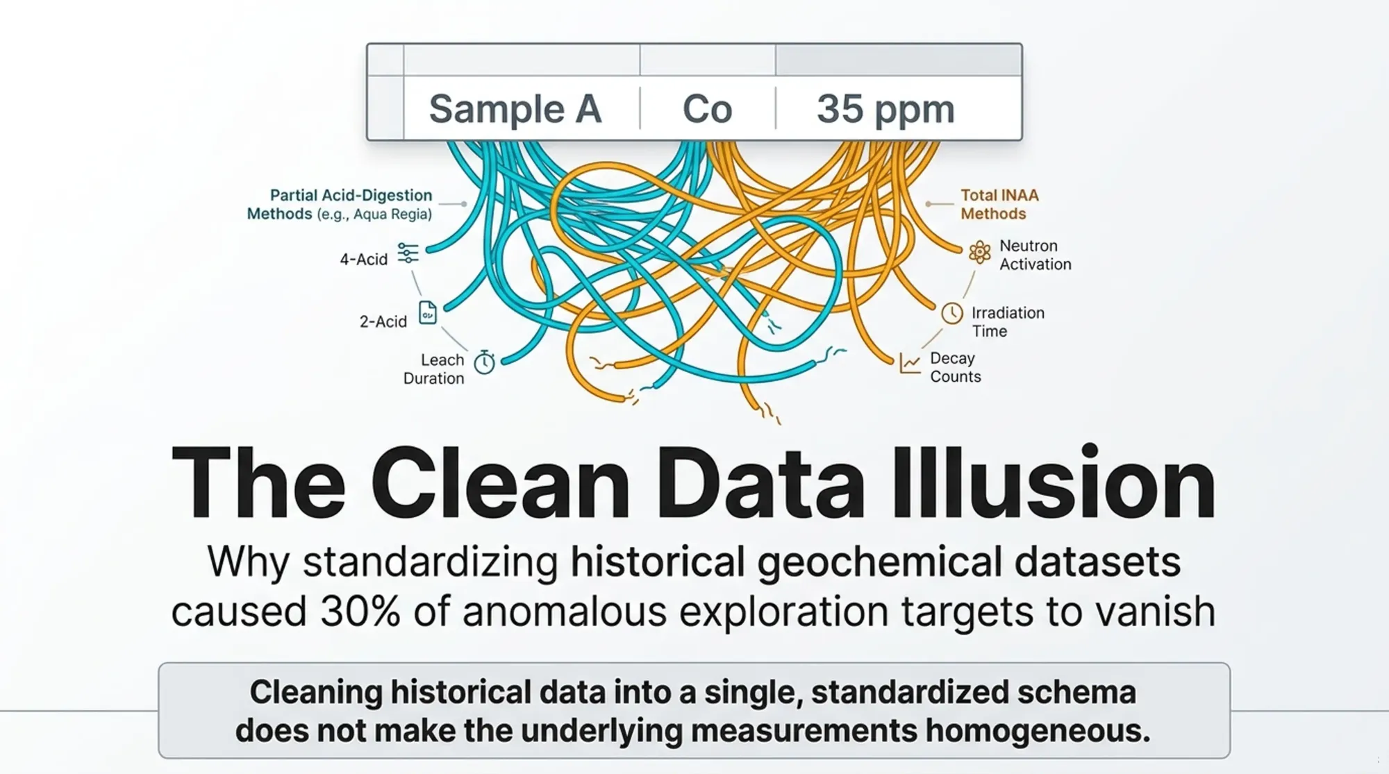
We tested what happens when historical geochemical assays produced by different analytical methods are treated as one population. In one regional cobalt dataset, changing nothing but how the analytical populations were standardised caused almost 30% of anomalous map cells to change classification.
If you have ever worked with a large historical geochemical dataset, the goal is usually to make it cleaner. Different files become one table. Units are standardised. Element names are reconciled. Old laboratory codes are decoded. Coordinates are cleaned up. Eventually, decades of messy historical assays start to look beautifully consistent.
And that is where a dangerous assumption can creep in.
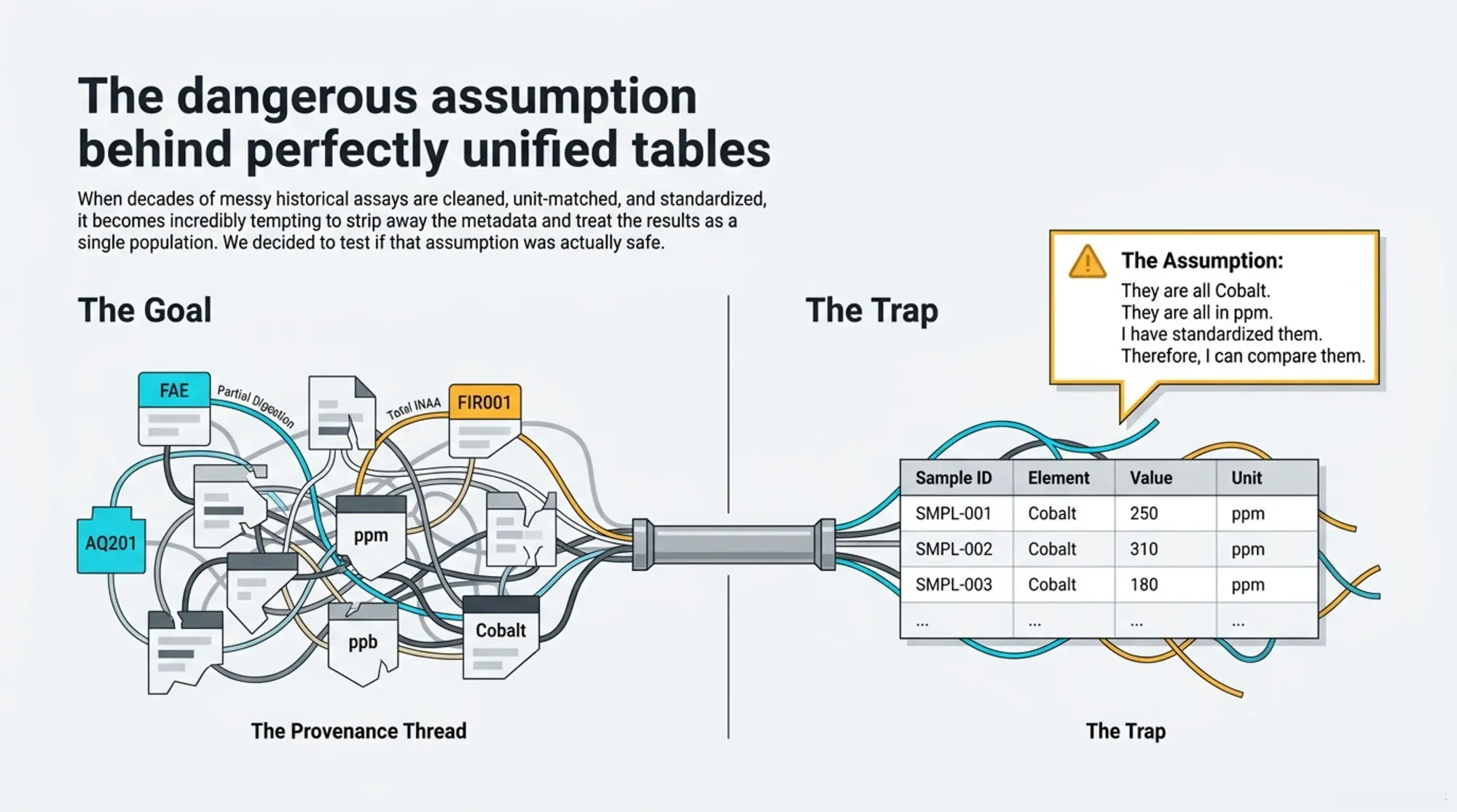
If two measurements are both labelled Co ppm, can we actually treat them as the same kind of measurement?
We decided to test it. Using 72,620 historical cobalt analyses from British Columbia, we compared what happens when different analytical populations are treated as one dataset versus when their analytical history is respected during standardisation.
The result surprised us. 29.5% of the anomalous map cells changed classification.
The assay results were the same. The coordinates were the same. The anomaly threshold was the same. The only thing we changed was the population used to decide what "unusual" meant.
Interestingly, we had not set out to study z-scores at all. This started with a much smaller problem: trying to work out what some old laboratory codes actually meant.
The experiment in one sentence: We wanted to know whether historical geochemical results could safely be treated as one population once the element names and units had been standardised.
It started with a much bigger problem: unifying global geochemistry
At RadiXplore, we have been working on a fairly ambitious problem: how do you make decades of public geochemical data from different jurisdictions usable together?
There is an enormous amount of geochemical information sitting in government databases, exploration reports and historical surveys around the world. If we want explorers, researchers or AI systems to reason across that information, the obvious first step is to bring it together.
But "bringing it together" is more complicated than putting everything into one database.
A single element can appear under different names. Units can vary. Detection limits change. Sample media are different. Laboratories use different preparation procedures, digestions and analytical finishes. And then there are the method codes.
Some are fairly easy to interpret. Others look more like FAE, FIR001, AQ201, ARU25MS or ME-MS61.
Some codes can be traced back to laboratory documentation. Some are self-describing. Some are highly specific to a particular laboratory, client or period. Others are extremely difficult to decode with confidence.
As part of our effort to make global geochemical data more useful, we started systematically working through these codes. For some of the more ambiguous ones, I shared examples on LinkedIn and asked people with practical laboratory and exploration experience for their interpretations.
One of the responses raised an important point: a laboratory method code should not necessarily be treated as a universal definition. Its meaning can depend on the laboratory, client, survey, time period and surrounding context.
That made us step back, because decoding the code was only the beginning. What happens after we decode it?
Once all of the data has been cleaned, converted into common units and placed into a structured table, it might eventually look something like this:
| Sample | Co (ppm) |
|---|---|
| A | 12 |
| B | 18 |
| C | 37 |
| D | 52 |
At that point, it becomes very tempting to forget where each number came from. They are all cobalt. They are all reported in ppm. If we want to screen a region for anomalous cobalt, we might log-transform the values, calculate z-scores and start looking for unusually high results.
The underlying assumption becomes:
They're all cobalt. They're all in ppm. I've standardised them. Therefore I can compare them.
We wanted to know whether that assumption was actually safe. More specifically, if we ignore analytical method and standardise all of the results together, can that change which samples or locations appear anomalous?
That became the study.
Finding a useful real-world experiment
We needed a dataset where we could test this properly, and we found one in the British Columbia Regional Geochemical Survey data.
For cobalt in stream sediments, our final dataset contained 72,620 usable analyses representing 44,616 physical samples, collected over several decades. Two major analytical populations dominated the data.
One group used an acid digestion followed by an atomic absorption finish. We treat this as a partial analytical method. The other used instrumental neutron activation analysis, or INAA, which involves no digestion and is treated as a total analytical method.
That alone would have given us something to investigate, but then we found something much more useful.
28,004 of the exact same physical samples had been analysed by both analytical populations.
That matters enormously. If one analytical method reports lower cobalt values than another, there is always an obvious alternative explanation: perhaps the two methods were simply used in different parts of the province. Method A might have been used over naturally lower-cobalt geology while Method B happened to be used in a mineralised region.
If that were true, the difference would have very little to do with analytical method.
Here, however, we could compare the same physical sample. Same stream sediment. Same location. Same cobalt. Two analytical histories.
The first surprise: the same sample did not give the same answer
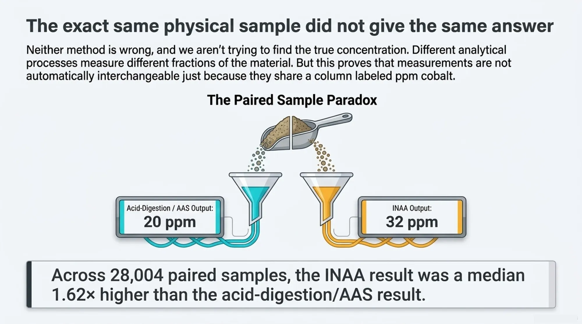
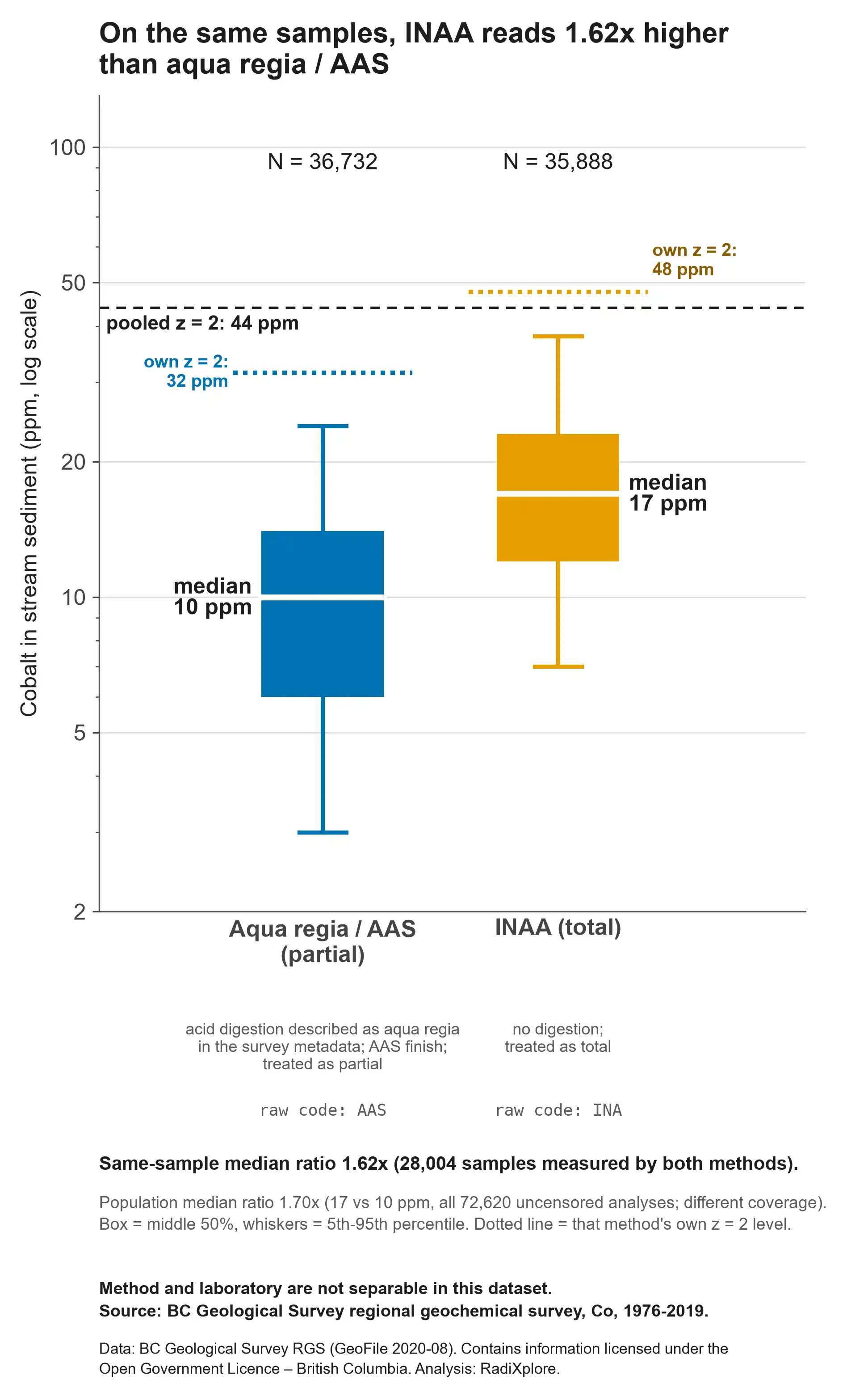
When we compared those 28,004 paired samples, the difference was clear. The INAA result was typically higher. Across the paired samples, the median relationship was approximately INAA = 1.62 × the acid-digestion/AAS result.
Imagine taking the same stream-sediment sample and getting 20 ppm cobalt using one analytical process and roughly 32 ppm cobalt using another.
That does not mean the first method is wrong, and it does not mean INAA is "better". We are not trying to establish the true cobalt concentration of each sample. Different analytical processes can measure different fractions of the material, so some disagreement is entirely reasonable.
But for our experiment, one thing was now clear:
The measurements were not automatically interchangeable just because they were both reported as ppm cobalt.
That led to the question we actually cared about. What happens if we treat them as interchangeable anyway?
Why a z-score does not solve the problem
Z-scores are commonly used in geochemistry because they make values easier to compare statistically. You do not need to worry about the formula to understand the important part.
A z-score is essentially asking:
How unusual is this value compared with the other values I gave you?
The phrase "the other values I gave you" is the important part.
Imagine one analytical method tends to produce cobalt results in a lower range while another tends to produce results in a higher range. If we combine both into one population, we create a new distribution. The lower-valued population affects the mean. The higher-valued population affects the mean. The spread of the combined dataset changes too.
Then every individual sample is judged against that combined population.
A z-score can standardise the distribution we give it. It cannot tell us whether those measurements should have been placed into the same population in the first place.
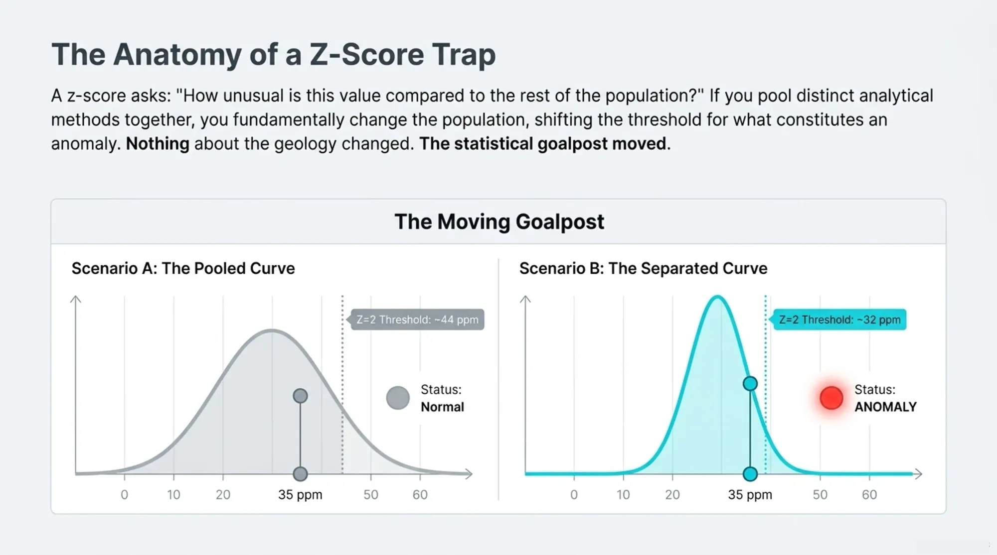
Our cobalt data illustrates this nicely. When all of the measurements were pooled together, a z-score of 2 corresponded to roughly 44 ppm cobalt. But when the two analytical populations were standardised independently, the equivalent approximate thresholds were 32 ppm for the acid-digestion/AAS population and 48 ppm for the INAA population.
That creates some interesting situations.
A simple example
Imagine an acid-digestion/AAS result of 35 ppm. Against the pooled threshold of roughly 44 ppm, it is not anomalous. But relative to other measurements from the same analytical population, where z=2 is roughly 32 ppm, it is anomalous.
Now imagine an INAA result of 45 ppm. Against the pooled population, it crosses the approximately 44 ppm threshold. Relative to the INAA population, where the equivalent threshold is closer to 48 ppm, it does not.
Nothing about the sample changed. Nothing about the geology changed. Nothing about the actual cobalt measurement changed.
We changed the statistical population used to decide what "unusual" meant.
That is the key to this entire experiment.
What happened when we put the anomalies back on the map?
Statistical differences are interesting, but explorers do not explore spreadsheets. They explore places.
So we took the same cobalt data and created two anomaly maps. In the first approach, all of the analytical results were pooled into one population before calculating the z-scores. In the second, the analytical populations were standardised separately.
Everything else stayed the same. The same 72,620 assay results, the same coordinates, the same map grid, the same anomaly definition and the same z-score threshold.
We then asked a very practical question: did the same places remain anomalous?
The answer was no.
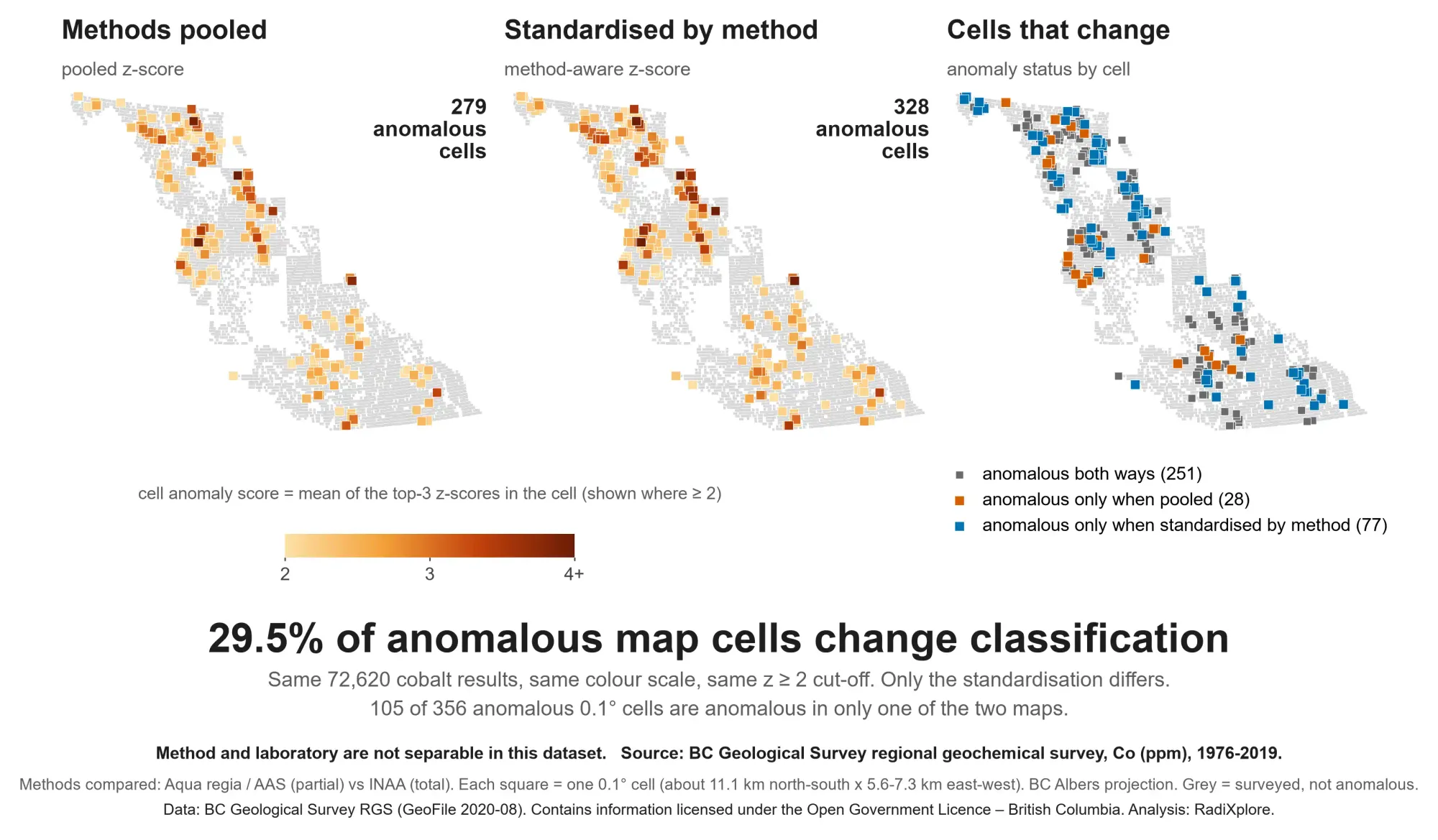
At our primary 0.1° map scale, there were 356 cells that were anomalous in at least one of the two approaches. Of those, 105 changed classification.
That is 29.5% of the anomalous map cells.
In the pooled analysis, there were 279 anomalous cells. In the method-aware analysis, there were 328. Of those, 251 appeared in both maps. Another 28 appeared only when the analytical populations were pooled, while 77 appeared only when the populations were standardised separately.
29.5% of anomalous map cells changed
Same measurements. Same locations. Same anomaly threshold. The only thing we changed was how the analytical populations were standardised.
The exact percentage changes depending on the grid size used, which is completely reasonable. Across the grid sizes we tested, roughly 20% to 35% of anomalous cells changed classification.
So 29.5% should not be treated as some universal correction factor for geochemical data. That is not the point. The important observation is that changing only how analytical populations were treated was enough to visibly change the anomaly map.
Then we tried to make the result disappear
A result that large immediately made us suspicious, so rather than stopping there, we started trying to break it.
Could the effect simply be caused by geography? Could duplicated analyses be exaggerating the result? Was our choice of grid size driving it? Was the z-score threshold arbitrary? Were detection limits affecting the distributions? What happens if we count physical samples rather than individual analytical rows? What if we randomly shuffle the method labels? What if we shuffle them while preserving the actual geography of the surveys?
We tested these questions in different ways. The effect became larger or smaller depending on the experiment, but it did not disappear.
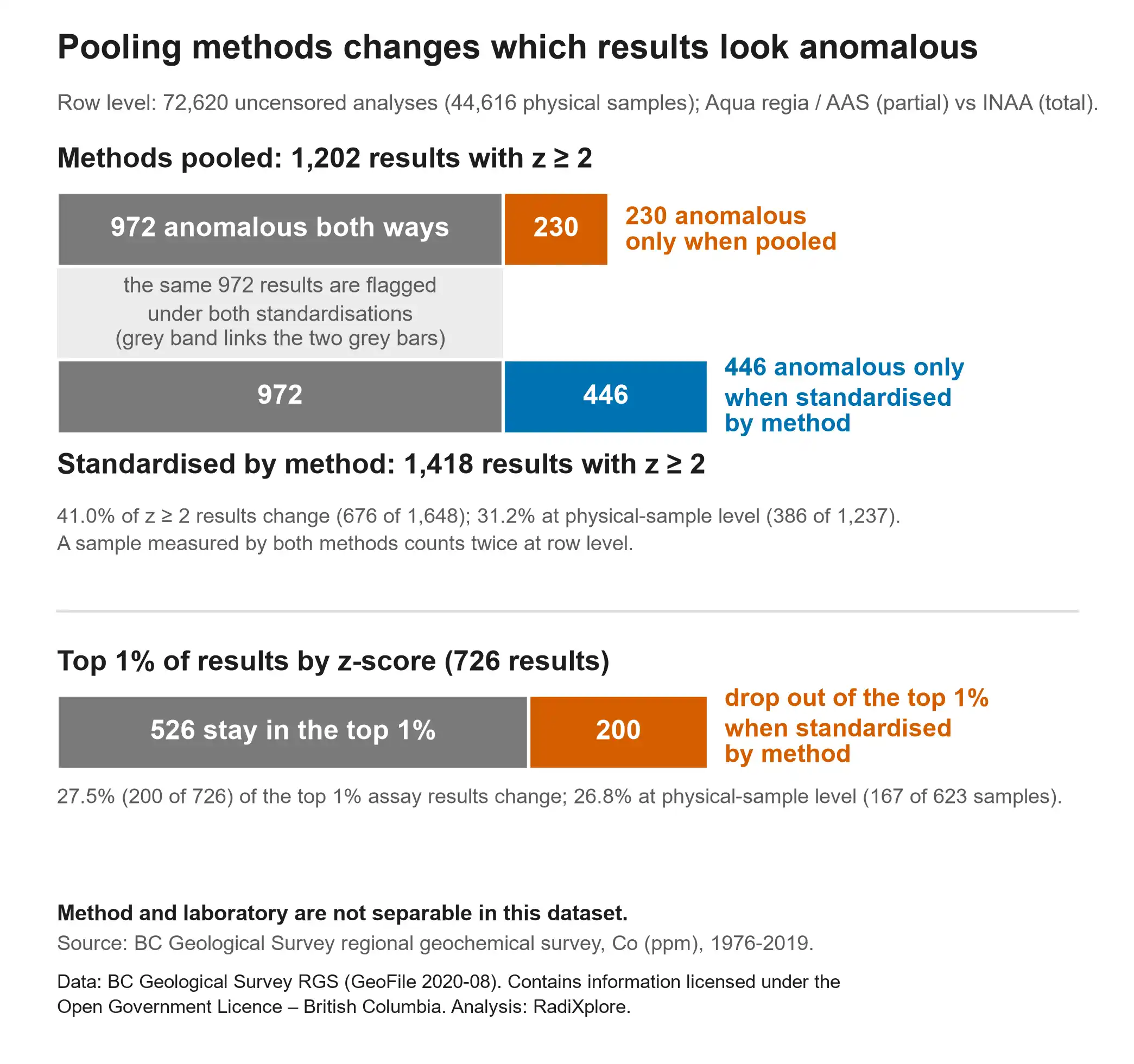
At a z ≥ 2 threshold, 41.0% of result rows classified as anomalous under either treatment changed classification. When we counted each physical sample only once, that fell to 31.2%.
We also ignored the z=2 threshold altogether and simply asked which results landed in the top 1%. Approximately 28% of that top 1% changed.
That matters because ranking assays is another very common workflow. If you are building a prospectivity model, or simply asking an AI system to surface the "most anomalous" historical results, your top-ranked list can change even though the underlying measurements have not.
We also performed placebo tests. When method labels were randomly shuffled, only a small proportion of anomaly classifications changed. Even when the shuffle preserved much of the real geographic structure, the observed effect remained substantially larger.
That gave us more confidence that we were not simply looking at a quirk of the map.
But there is an important limitation.
What this experiment cannot tell us
Analytical method was not the only thing that changed over the decades represented by this dataset. Laboratories changed. Survey programs changed. Time periods changed. Sampling campaigns changed.
In this particular cobalt dataset, laboratory and analytical method cannot be fully separated because no individual laboratory ran both of our major analytical populations.
That means we should not describe everything we observed as a pure "method effect". A more accurate description is an analytical-population effect. The method matters, but it exists alongside laboratory, survey and historical context.
We also cannot use this study to say which result is "correct". There is no certified reference value for these individual field samples, and that was never the question we were asking.
The question was much simpler:
Are these measurements similar enough that we can safely pretend their analytical history does not exist?
In this cobalt dataset, the answer was clearly no.
Does this mean different analytical methods should never be combined?
No. And this is one of the most important parts of the experiment.
If we had stopped at the cobalt result, it would be easy to walk away with the conclusion that historical assays from different methods should simply never be pooled. That would also be wrong.
We deliberately looked for a case where different analytical populations behaved similarly, and we found one in Canadian lake-sediment copper data.
In that dataset, 18,320 physical samples had paired measurements produced using aqua-regia and four-acid analytical approaches. This time, the measurements agreed very closely. Their median ratio was approximately 1.08, and their Spearman correlation was 0.95.
In other words, the two analytical populations behaved much more similarly. In that case, separating the populations before standardisation was far less consequential.
And that gave us what I think is the most useful conclusion of the entire experiment:
Analytical methods do not always matter enough to change your interpretation. But you cannot know that if you have already thrown the method metadata away.
The answer is not never combine methods.
The answer is do not assume they are comparable without checking.
Why this matters even more when AI enters the workflow
None of this is uniquely an AI problem. A geologist working in a spreadsheet can make exactly the same mistake.
But AI changes the scale.
We can now process geochemical datasets containing millions or tens of millions of observations. We can ask machine-learning models to rank anomalous areas. We can build prospectivity models across entire jurisdictions. We can give agents access to historical assays, drilling data, reports, maps and geological context.
That is incredibly powerful, but it also means assumptions that once affected a spreadsheet can now propagate across entire datasets.
An AI system does not inherently know that two columns both called Co_ppm may represent measurements produced using different digestions, instruments, detection limits, laboratories or survey programs.
There is an even more subtle risk. A sufficiently capable model may learn those differences extremely well.
Suppose one analytical method dominates a particular decade. Another method dominates a specific survey program. One laboratory worked mainly in a certain part of a jurisdiction. The model may discover that those analytical characteristics are highly predictive of mineralisation.
Statistically, that relationship might be real.
But the model could partly be learning how the data was collected, rather than what the geology is telling us.
That is why provenance becomes more important as our ability to analyse data improves. The more powerful the model, the less comfortable I am with giving it a beautifully clean table whose history has been stripped away.
What this changed for us at RadiXplore
This experiment started because we were trying to decode old laboratory method codes. At first, the method field looked like another piece of messy metadata that needed to be cleaned before we could get to the interesting geology.
We now look at it very differently.
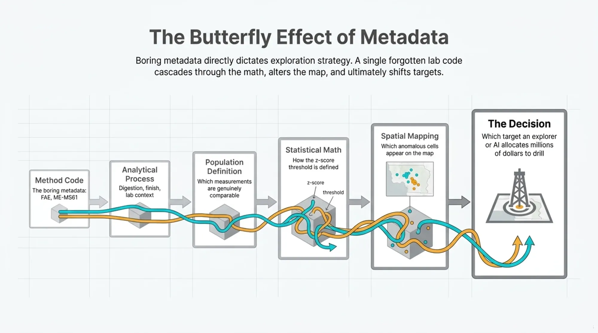
A method code points to an analytical process. That process affects which measurements may reasonably be compared. That decision shapes the statistical population. The statistical population affects which samples appear anomalous. Those anomalies affect which locations appear interesting. And those locations may ultimately influence which targets an explorer, or an AI system, pays attention to.
That means the boring metadata can eventually influence an exploration decision.
As we continue working towards more unified geochemical datasets, we increasingly want to preserve information such as sample medium, sample preparation, digestion or extraction, analytical finish, laboratory, detection limit, survey or program, analysis date, original method code and confidence in the method interpretation.
Not because every analysis needs to be separated by every possible variable. Sometimes those differences will barely matter. Our copper example demonstrates that.
But if you retain the provenance, you can test whether they matter.
If you remove it, you no longer have that option.
So what did we actually learn?
We did not learn that z-scores are bad. The z-score did exactly what we asked it to do.
The assumption was in the population we gave it.
We did not learn that INAA is better than acid digestion. We did not learn that all analytical methods must always be separated. And we certainly did not discover a universal 29.5% error rate for historical geochemistry.
What we learned was more fundamental.
Cleaning historical data into the same schema does not make the underlying measurements homogeneous.
A table can look perfectly consistent while still containing decades of analytical history. The element can be the same. The units can be the same. The coordinates can be the same. The measurement processes can still be very different.
Sometimes that distinction may have almost no effect on the geological interpretation.
Sometimes, as we saw here, it can change almost a third of the anomalous map cells.
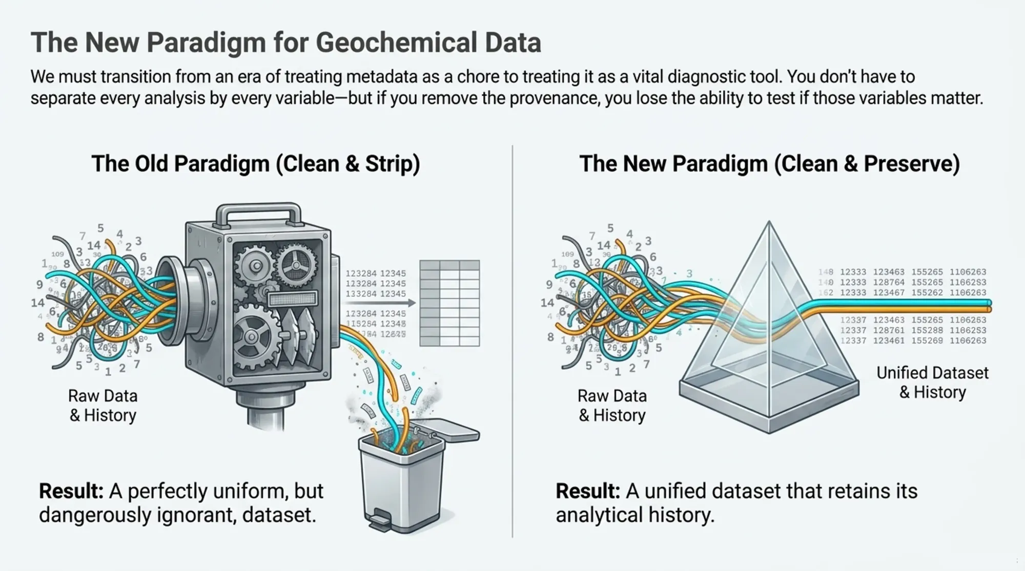
And we only discovered that because we kept the analytical history attached to the data.
For the technically curious
Dataset
The primary study uses British Columbia Regional Geochemical Survey stream-sediment cobalt data spanning 1976 to 2019. The final analysis contains 72,620 uncensored analytical results, 44,616 physical samples and 28,004 physical samples analysed by both major analytical populations.
Analytical populations
The two dominant populations are an aqua-regia/acid-digestion plus atomic absorption population, treated as partial, and instrumental neutron activation analysis, or INAA, treated as total.
Standardisation
Cobalt values were log-transformed before z-score standardisation. We compared pooled standardisation, where both analytical populations were treated as one distribution, with analytical-population-aware standardisation, where each population was standardised independently.
Mapping
For the primary spatial comparison, results were aggregated into 0.1° cells. The same assay data, coordinates, aggregation procedure and z ≥ 2 anomaly definition were used in both treatments. Only the standardisation strategy changed.
Robustness checks
The analysis also examined alternative grid sizes, different anomaly thresholds, row-level versus physical-sample-level treatment, top-percentile rankings, censoring and detection-limit effects, random method-label shuffles, geographically constrained placebo shuffles, and laboratory and temporal structure.
Important limitations
This study covers one primary analyte, one sample medium and one regional database. Analytical method and laboratory cannot be independently identified in the primary cobalt case. The analysis does not determine which analytical measurement is closer to the "true" cobalt concentration of an individual sample.
The 29.5% map result is specific to the selected dataset, threshold and map scale and should not be generalised as a universal correction factor.
Data source
Primary analysis based on British Columbia Geological Survey Regional Geochemical Survey data.
Data contains information licensed under the Open Government Licence – British Columbia.
Working with historical geochemical data?
If you are building prospectivity models, analysing regional datasets or trying to make decades of assays comparable, we would be interested to hear how you are approaching the same problem.